 하나씩 점을 찍어 나가며
이 글은Future Sales Prediction: playground커널의 리뷰입니다.
코드 및 아이디어는 모두 커널의 원 제작자에게 있으며, 이 글은 해당 커널을 좀 더 이해하기 쉽게하기 위한 리뷰입니다.
5. Data Preparation
Feature Creation 도 끝났고, 이제 본격적으로 모델을 만들어보려고 합니다.
그 전에, train dataset 을 모델에 들어갈 모양으로 만들어보겠습니다.
최종적으로는 지금까지 만든 모든 feature 들을 모두 합친 데이터프레임을 만들건데, 이 과정 중에 메모리가 매우 많이 사용될 수 있습니다.
따라서, 먼저 데이터프레임을 최대한 메모리 최적화 시켜놔야 합니다.
예를 들면, category feature는 데이터 타입을 category 화 시켜줘야하고, int64 타입의 feature 지만 int8 로도 충분히 커버가능한 경우 int8로 바꿔주는 식으로 말입니다.
이런 귀찮은 작업을 사전에 누군가가 함수로 만들어놓았습니다.
우리는 단지 이 함수를 가져와 쓰면됩니다.
함수가 어떻게 작동하는지 몰라도, 인자로 데이터프레임을 넘겨주면 알아서 최적화 시켜줄 것입니다.
# Memory saving function credit to https://www.kaggle.com/gemartin/load-data-reduce-memory-usage
def reduce_mem_usage(df):
    """ iterate through all the columns of a dataframe and modify the data type
        to reduce memory usage.
    """
    start_mem = df.memory_usage().sum() / 1024**2

    for col in df.columns:
        col_type = df[col].dtype

        if col_type != object:
            c_min = df[col].min()
            c_max = df[col].max()
            if str(col_type)[:3] == 'int':
                if c_min > np.iinfo(np.int8).min and c_max < np.iinfo(np.int8).max:
                    df[col] = df[col].astype(np.int8)
                elif c_min > np.iinfo(np.int16).min and c_max < np.iinfo(np.int16).max:
                    df[col] = df[col].astype(np.int16)
                elif c_min > np.iinfo(np.int32).min and c_max < np.iinfo(np.int32).max:
                    df[col] = df[col].astype(np.int32)
                elif c_min > np.iinfo(np.int64).min and c_max < np.iinfo(np.int64).max:
                    df[col] = df[col].astype(np.int64)
            else:
                #if c_min > np.finfo(np.float16).min and c_max < np.finfo(np.float16).max:
                #    df[col] = df[col].astype(np.float16)
                #el
                if c_min > np.finfo(np.float32).min and c_max < np.finfo(np.float32).max:
                    df[col] = df[col].astype(np.float32)
                else:
                    df[col] = df[col].astype(np.float64)
        #else:
            #df[col] = df[col].astype('category')

    end_mem = df.memory_usage().sum() / 1024**2
    print('Memory usage of dataframe is {:.2f} MB --> {:.2f} MB (Decreased by {:.1f}%)'.format(
        start_mem, end_mem, 100 * (start_mem - end_mem) / start_mem))
    return df
다음으로, 우리가 지금까지 만든 feature들의 데이터프레임을 한 군데로 합쳐줄 함수를 정의합니다.
또 이 과정중에, month 와 day feature 도 추가해주고, 결측치는 0으로 채워줍니다.
def mergeFeature(df):
    df = pd.merge(df, items, on=['item_id'], how='left').drop('item_group', axis=1)
    df = pd.merge(df, item_cats, on=['item_category_id'], how='left')
    df = pd.merge(df, shops, on=['shop_id'], how='left')

    df = pd.merge(df, train_shop, on=['shop_id','item_id'], how='left')
    df = pd.merge(df, train_shop_cat, on=['shop_id','item_group'], how='left')
    df = pd.merge(df, train_prev, on=['date_block_num','shop_id','item_id'], how='left')
    df = pd.merge(df, train_cat_prev, on=['date_block_num','shop_id','item_group'], how='left')
    df = pd.merge(df, train_ema_prev, on=['date_block_num','shop_id','item_id'], how='left')

    df['month'] = df['date_block_num'] % 12
    days = pd.Series([31,28,31,30,31,30,31,31,30,31,30,31])
    df['days'] = df['month'].map(days).astype(np.int8)

    df.drop(['shop_id','shop_name','item_id','item_name','item_category_id','item_category_name','item_group'], axis=1, inplace=True)
    df.fillna(0.0, inplace=True)
    return reduce_mem_usage(df)
이제 모델 훈련에 들어갈 데이터셋, train set 을 만들어줍니다.
이 때, 전 기간의 모든 데이터셋을 사용하지 않고 초반의 12개월 후의 데이터만 사용합니다.
왜냐하면, 현재 우리 training feature 에는, 12개월 전의 값들(order_prev12 와 같은)이 들어가 있습니다.
즉, 12개월 전의 data, 예를 들어 초반 6월의 데이터에는 12개월 전의 데이터가 없는거지요. 따라서, 12개월 후의 데이터만을 사용해야, 온전한 feature 값을 얻을 수 있습니다.
한편, 이상치에 로버스트하게 하기위해, 기존 이상치 값들을 0 혹은 20으로 바꿔줍니다.
train_set = train_monthly[train_monthly['date_block_num'] >= 12]

train_set = pd.merge(train_set, train_price_a, on=['date_block_num','shop_id','item_id'], how='left')
train_set = mergeFeature(train_set)

train_set = train_set.join(pd.DataFrame(train_set.pop('item_order'))) # move to last column
X_train = train_set.drop(['item_cnt'], axis=1)

Y_train = train_set['item_cnt'].clip(0.,20.)
X_train.head()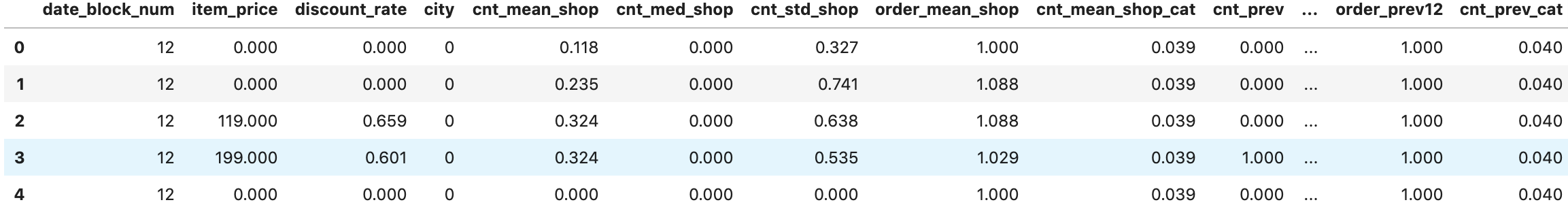
마찬가지로 test set 에도 동일한 작업을 해줍니다.
test_set = test.copy()
test_set['date_block_num'] = 34

test_set = pd.merge(test_set, test_price_a, on=['shop_id','item_id'], how='left')
test_set = mergeFeature(test_set)

test_set['item_order'] = test_set['cnt_ema_s_prev'] #order_prev
test_set.loc[test_set['item_order'] == 0, 'item_order'] = 1

X_test = test_set.drop(['ID'], axis=1)
X_test.head()

assert(X_train.columns.isin(X_test.columns).all())
6. Prediction
이전에 우리가 사용할 모델은 lgb 라고 했습니다.
모델에 필요한 라이브러리들과 lgb model 에 들어갈 파라미터들을 설정해줍니다.
그리고, KFold 를 사용하여 train 시킬 것인데, 같은 달의 데이터가 쪼개지지 않고 온전히 train 혹은 validation set 에 들어가게 하기위해서, group KFold 를 사용하겠습니다.
group KFold 는 이런 목적으로 등장한 KFold 방법인데, 아래 링크를 통해 보시면, 어떤건지 아실 수 있습니다.
참고로, 저도 이번에 처음 알았습니다.
sklearn 공식 docu : sklearn.model_selection.GroupKFold
게으른 우루루님 블로그 : 다양한 교차 검증 방법
from sklearn import linear_model, preprocessing
from sklearn.model_selection import GroupKFold
import lightgbm as lgb

params={'learning_rate': 0.05,
        'objective':'regression',
        'metric':'rmse',
        'num_leaves': 64,
        'verbose': 1,
        'random_state':42,
        'bagging_fraction': 1,
        'feature_fraction': 1
       }

folds = GroupKFold(n_splits=6)
oof_preds = np.zeros(X_train.shape[0])
sub_preds = np.zeros(X_test.shape[0])
oof_preds 에는 훈련한 모델에 validation dataset 을 입력했을 때 나오는 출력 값이,sub_preds 에는 훈련한 모델에 test dataset 을 입력했을 때 나오는 출력 값이 들어갑니다.
기본적으로 0으로 다 초기화시켜놓은 뒤, 인덱스를 통해 접근해서 0이 예측 값으로 바꾸게 할 예정입니다.
이제 다음과 같이 예측합니다.
for fold_, (trn_, val_) in enumerate(folds.split(X_train, Y_train, X_train['date_block_num'])):
    trn_x, trn_y = X_train.iloc[trn_], Y_train[trn_]
    val_x, val_y = X_train.iloc[val_], Y_train[val_]

    reg = lgb.LGBMRegressor(**params, n_estimators=3000)
    reg.fit(trn_x, trn_y, eval_set=[(val_x, val_y)], early_stopping_rounds=50, verbose=500)

    oof_preds[val_] = reg.predict(val_x.values, num_iteration=reg.best_iteration_)
    sub_preds += reg.predict(X_test.values, num_iteration=reg.best_iteration_) / folds.n_splits
먼저 위 코드를 설명하면 이렇습니다.
- 이전에
folds = GroupKFold(n_splits=6)로 주었기 때문에, 총 6개의 (train / validaiton) 구성이 생기게 되고, 반복문도 6번 돌게 됩니다. trn_과val_에는 현재 (train / validaiton) 구성에서, train에 들어갈 데이터의 index들, validation에 들어갈 데이터의 index들이 담깁니다.- train 으로 먼저 훈련시킨 모델
reg에 validation dataset으로 prediction 한 값으로oof_preds[val_]을 계속해서 업데이트 시킵니다. - 마찬가지로
sub_preds에도 test dataset으로 prediction 한 값을 계속해서 더해줍니다. 이러한 과정을 6번 동안 하므로, 총 6번 더 해지게되는데, 이를 6(folds.n_splits)으로 나눠줌으로써 올바른 값을 넣어줍니다.
코드를 돌리면 이제 다음과 같이 출력됩니다.
Training until validation scores don't improve for 50 rounds.
[500]    valid_0's rmse: 0.209647
[1000]    valid_0's rmse: 0.207681
Early stopping, best iteration is:
[1018]    valid_0's rmse: 0.207633
Training until validation scores don't improve for 50 rounds.
[500]    valid_0's rmse: 0.206711
[1000]    valid_0's rmse: 0.205003
Early stopping, best iteration is:
[1294]    valid_0's rmse: 0.20464
Training until validation scores don't improve for 50 rounds.
[500]    valid_0's rmse: 0.208489
[1000]    valid_0's rmse: 0.205751
Early stopping, best iteration is:
[1275]    valid_0's rmse: 0.20516
Training until validation scores don't improve for 50 rounds.
[500]    valid_0's rmse: 0.186031
Early stopping, best iteration is:
[607]    valid_0's rmse: 0.185691
Training until validation scores don't improve for 50 rounds.
[500]    valid_0's rmse: 0.15861
Early stopping, best iteration is:
[463]    valid_0's rmse: 0.158591
Training until validation scores don't improve for 50 rounds.
[500]    valid_0's rmse: 0.186485
Early stopping, best iteration is:
[547]    valid_0's rmse: 0.18632
rmse 가 점점 감소하는 것을 볼 수 있습니다.
이제 우리 모델이 잘 훈련되었는지, 확인해보겠습니다.
print('RMSE:', np.sqrt(metrics.mean_squared_error(Y_train, oof_preds.clip(0.,20.))))RMSE: 0.19348729089786737꽤 괜찮게 나온 것 같습니다.
각 모델의 피처들의 중요도가 어떤지 한번 살펴보겠습니다.
# Plot feature importance
feature_importance = reg.feature_importances_
feature_importance = 100.0 * (feature_importance / feature_importance.max())
sorted_idx = np.argsort(feature_importance)
pos = np.arange(sorted_idx.shape[0]) + .5

plt.figure(figsize=(12,6))
plt.barh(pos, feature_importance[sorted_idx], align='center')
plt.yticks(pos, X_train.columns[sorted_idx])
plt.xlabel('Relative Importance')
plt.title('Variable Importance')
plt.show()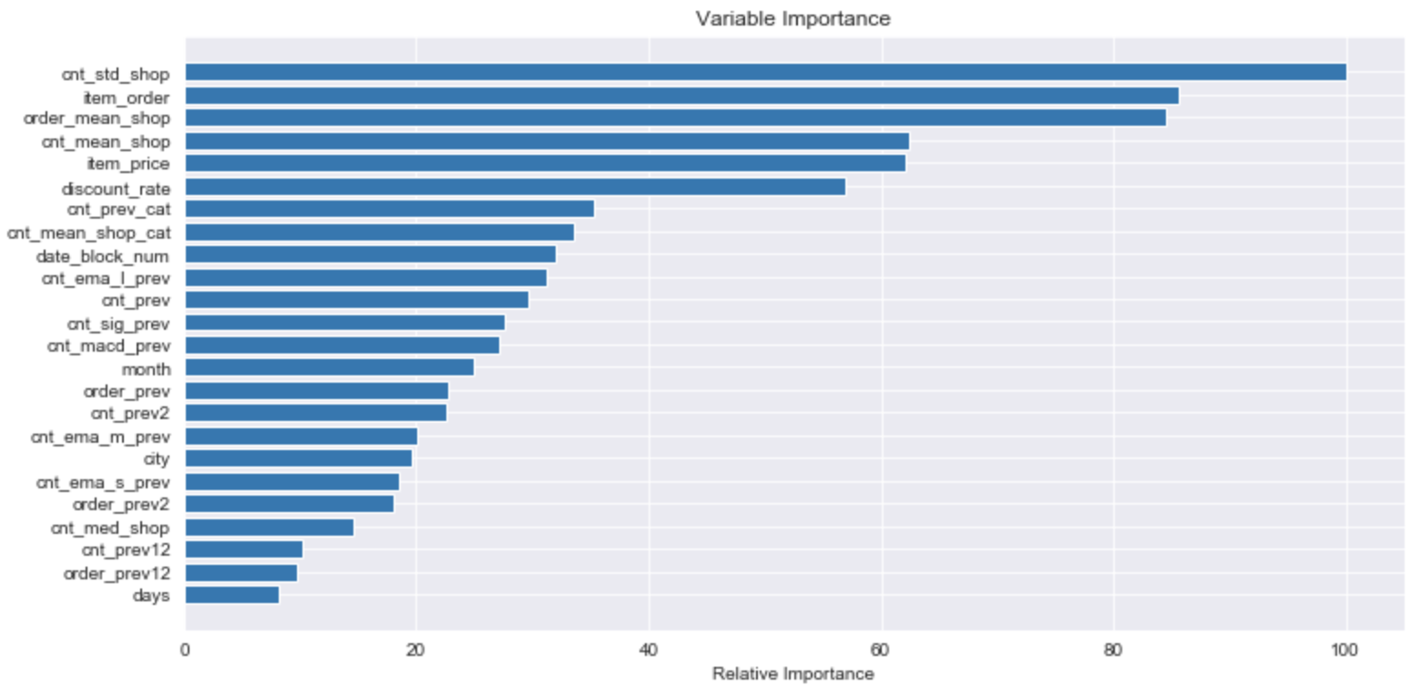
이 전에 feature importance 를 살펴본적 있으므로, 별다른 설명은 하지 않겠습니다.
다만, 이렇게 볼 수 있다. 정도로만 살펴보았습니다.
feature의 구체적인 해석은 또 별게의 문제인 듯 합니다.
이제 끝났습니다.
최종적으로 Kaggle 에 제출할 submission 파일을 만듭니다.
우리는 이상치에 민감하지 않은 모델이었으므로, 마찬가지로 0~20사이로 값을 만들어 내보냅니다.
pred_cnt = sub_preds
result = pd.DataFrame({
    "ID": test["ID"],
    "item_cnt_month": pred_cnt.clip(0. ,20.)
})
result.to_csv("submission.csv", index=False)
이제 만들어진 submission.csv 를 Kaggle 에 제출하면 끝이납니다.
후기
이번 커널은 그래도 생각보다 간결하고, 직관적이며 코드가 그렇게 어렵지 않았다고 생각합니다.
pandas 에서 .clip() 이 무엇인지, 어떻게 쓰는건지도 알 수 있었고,
Feature 만드는 것을 각자 따로한 뒤, 나중에 합치는 테크닉들도 배울 수 있었네요.
한편, 다음에 대해 공부해본 뒤, 나중에 기록해봐야겠단 생각이 들었습니다.
- light gbm model
- ensemble
- bagging vs boosting
- 일반적인 boosting model.
- gradient boosting model.
- 보다 다양한 K-Fold 방법과 사용 시기
이번 커널 리뷰는 이 글로 마칩니다.
'데이터와 함께 탱고를 > 커널 공부하기' 카테고리의 다른 글
| [Predict Future Sales] xgboost 커널 리뷰 (4) | 2019.08.01 |
|---|---|
| [Predict Future Sales] playground 커널 리뷰 1 (2) | 2019.07.28 |
| [Predict Future Sales] playground 커널 리뷰 0 (0) | 2019.07.28 |
| [Predict Future Sales] 대회 및 데이터 소개 (1) | 2019.07.27 |
| 커널을 공부해본다. (0) | 2019.07.25 |


