 하나씩 점을 찍어 나가며
이번에 살펴볼 커널은 Feature engineering, xgboost 입니다.
Voting 수 2위에다가, RMSE public score 도 0.90684 로, 저번에 리뷰한 커널보다 점수가 높습니다.
전반적인 흐름은 저번과 비슷합니다.
먼저, Feature 를 만드는데 중점을 두고, 모델을 통해 학습하여 예측합니다.
다만 이번에는 저번에 리뷰한 커널보다 Feature 수가 훨씬 많고, 모델도 xgboost 를 사용합니다.
서론
대회 소개 및 목표
한 마디로 말해, 기존의 Sales 데이터를 가지고, 미래의 Sales 량을 예측하는 대회입니다.
정확히는, 2013년 1월~2015년 10월의 모든 shop 내 item들의 하루 단위의 세일즈량이 주어지고,
이후 다음 달(2015년 11월)의 각 shop의 각각의 item 세일즈량의 총 합을 예측해야 합니다.
진행순서
Part1 에서는 모델에 들어갈 데이터프레임 형태로 만든 후, 필요해보이는 Feature 를 만드는데 중점을 둡니다.
큰 그림으로 보면, 다음과 같은 Feature 들을 만들 것입니다.
- 월별 각 상점의 상품 세일즈량
- 세분화된 아이템 카테고리
- 상점이 위치한 도시
- 현재 월 기준, 이전 달들의 각종 평균 값
- 현재 월, 일
- 상품이 마지막으로 팔리고 지난 월 수.
- 상품이 맨 처음 팔리고 지난 월 수.
Part2 에서는 xgboost 모델을 가지고, 모델을 훈련시킬 것입니다.
훈련 후, 실제로 Feature 들이 어느정도의 중요도를 가지는지 살펴보겠습니다.
Part 1, Perfect Features
Data and Library Load
먼저, 필요한 라이브러리들을 import 하고, 들어가기 전 기본적인 설정을 해줍니다.
# 데이터 조작을 위한 프레임워크 numpy, pandas.
import numpy as np
import pandas as pd
pd.set_option('display.max_rows', 500)
pd.set_option('display.max_columns', 100)

# 특별한 데이터 조작을 위한 라이브러리 add on.
from itertools import product
from sklearn.preprocessing import LabelEncoder

# 사용할 시각화 툴 seaborn, pyplot.
import seaborn as sns
import matplotlib.pyplot as plt
%matplotlib inline

# model은 xgboost을 사용합니다.
from xgboost import XGBRegressor
from xgboost import plot_importance

def plot_features(booster, figsize):
    fig, ax = plt.subplots(1,1,figsize=figsize)
    return plot_importance(booster=booster, ax=ax)

# 메모리, 실행시간, 데이터 저장 등, 기타 목적을 위한 라이브러리들.
import time
import sys
import gc
import pickle
sys.version_info
sys.version_info(major=3, minor=6, micro=8, releaselevel='final', serial=0)데이터를 읽어옵니다.
items = pd.read_csv('../input/items.csv')
shops = pd.read_csv('../input/shops.csv')
cats = pd.read_csv('../input/item_categories.csv')
train = pd.read_csv('../input/sales_train.csv')
# set index to ID to avoid droping it later
test  = pd.read_csv('../input/test.csv').set_index('ID')
각 데이터에 대한 소개는 이전 포스팅에서 언급한 적이 있으므로, 생략하겠습니다.
Outliers
가장 먼저, 이상값, 극단값이 있는지 먼저 살펴보겠습니다.
데이터 features 중, item_price 와 item_cnt_day 를 살펴보면 다음과 같습니다.
plt.figure(figsize=(10,4))
plt.xlim(-100, 3000)
sns.boxplot(x=train.item_cnt_day)

plt.figure(figsize=(10,4))
plt.xlim(train.item_price.min(), train.item_price.max()*1.1)
sns.boxplot(x=train.item_price)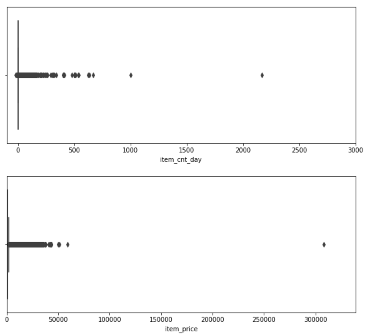
각 플롯에 보이는 매우 극단적인 값들이 보입니다.
이 데이터들은 일단 데이터셋에서 제외시키도록 하겠습니다.
train = train[train.item_price<100000]
train = train[train.item_cnt_day<1001]
한편, price 도 살펴보겠습니다.
plt.figure(figsize=(10,4))
plt.xlim(train.item_price.min(), 0)
sns.boxplot(x=train.item_price)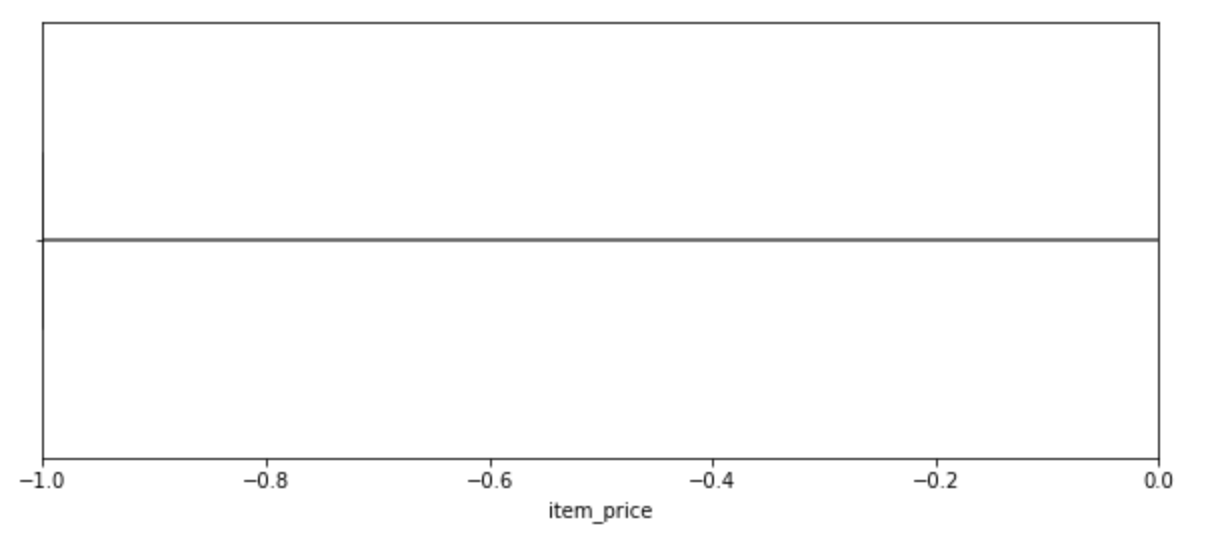
price가 0 미만인 '이상 값' 이 존재합니다.
이 값을 해당 상품의 전 기간의 가격들 중, 중간값으로 바꿔주겠습니다.
median = train[(train.shop_id==32)&(train.item_id==2973)&(train.date_block_num==4)&(train.item_price>0)].item_price.median()
train.loc[train.item_price<0, 'item_price'] = median
또 살펴본 결과, 일부 shop_id 가 shop_name 하고 맞지않는 데이터가 있었습니다.
이 값들도 고쳐주겠습니다.
# Якутск Орджоникидзе, 56
train.loc[train.shop_id == 0, 'shop_id'] = 57
test.loc[test.shop_id == 0, 'shop_id'] = 57
# Якутск ТЦ "Центральный"
train.loc[train.shop_id == 1, 'shop_id'] = 58
test.loc[test.shop_id == 1, 'shop_id'] = 58
# Жуковский ул. Чкалова 39м²
train.loc[train.shop_id == 10, 'shop_id'] = 11
test.loc[test.shop_id == 10, 'shop_id'] = 11
Shops/Cats/Items preprocessing
shops, cats, items 에 있는 데이터로, 일부 새로운 Feature 를 만들어볼까 합니다.
먼저, shops 부터 보겠습니다.
shops.head()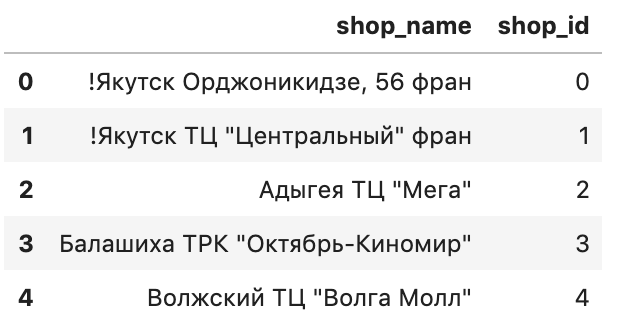
Shops를 보면, shop_name의 첫 번째 단어가, 해당 상점이 해당하는 도시 이름입니다.
예를 들어, 상점 이름이 "마포구 스타벅스" 식으로 되어있는 것이죠.
따라서, shop_name 으로 부터, 도시 이름을 뽑아내고, 이를 새로운 Feature 로 둘 수 있습니다.
이를 city 라고 하고, 이를 Label encoding 한 것을 city_code 라고 하겠습니다.
# 일부 데이터의 shop_name 이 통일되지 않는 게 있습니다. 이를 보정해줍니다.
shops.loc[shops.shop_name == 'Сергиев Посад ТЦ "7Я"', 'shop_name'] = 'СергиевПосад ТЦ "7Я"'

# shop_name 으로부터 city 를 추출하여 새로운 Feature를 만듭니다.
shops['city'] = shops['shop_name'].str.split(' ').map(lambda x: x[0])
shops.loc[shops.city == '!Якутск', 'city'] = 'Якутск' # Якутск 역시, 통일되지 않은 도시라 보정해줍니다.

# city 를 LabelEncoder 로 encoding 하여 새로운 Feature를 만듭니다.
shops['city_code'] = LabelEncoder().fit_transform(shops['city'])
shops = shops[['shop_id','city_code']]
이번엔 Cats를 보겠습니다.
cats.head()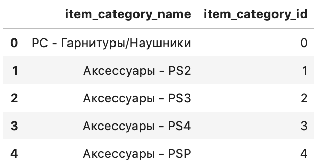
item_category_name 를 보면, 첫 번째 단어와 두 번째 단어가 모두 서브 카테고리 이름임을 알 수 있습니다.
예를 들어, 카테고리 이름이 "전자기기-노트북" 식으로 되어있는거죠.
마찬가지로, 여기서 두 개의 카테고리를 뽑아내어 새로운 Feature 로 만들겠습니다.
이 때, 첫 번째 카테고리를 type, 두 번째 카테고리를 subtype 이라고 하겠습니다.
이를 Label encoding 한 것을 마찬가지로, type_code, subtype_code 라고 하겠습니다.
cats['split'] = cats['item_category_name'].str.split('-')
cats['type'] = cats['split'].map(lambda x: x[0].strip())
cats['type_code'] = LabelEncoder().fit_transform(cats['type'])

# if subtype is nan then type
cats['subtype'] = cats['split'].map(lambda x: x[1].strip() if len(x) > 1 else x[0].strip())
cats['subtype_code'] = LabelEncoder().fit_transform(cats['subtype'])
cats = cats[['item_category_id','type_code', 'subtype_code']]
items 에는, 별달리 뽑을게 없는 듯 합니다.
우리는 item_id 만 쓸 것이므로, item_name 은 지워놓겠습니다.
items.drop(['item_name'], axis=1, inplace=True)Monthly sales
테스트 데이터셋은 34번째 달(우리가 예측해야하는 달)의 상점x상품의 꼴로 되어있습니다.
어떻게 생겼나 실제로 보겠습니다.
test.head()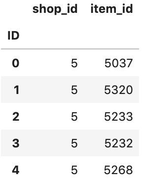
한편, train 데이터셋에는 없고, test 데이터셋에만 존재하는 상품이 있을 수 있습니다.
(이런 상품의 개수, test 데이터셋에 존재하는 상품 수, 테스트 데이터셋 크기) 를 한 번 보겠습니다.
len(list(set(test.item_id) - set(test.item_id).intersection(set(train.item_id)))), len(list(set(test.item_id))), len(test)(363, 5100, 214200)먼저 우리는, (월, 상점, 상품) 을 기준으로하는 데이터프레임을 만들필요가 있습니다.
우리가 예측하려고 하는 것은 개별 (월, 상점, 상품) 의 상품 판매량이니깐요.
이를 위해, 모든 경우의 월(모든 기간), 상점(모든 상점), 상품(모든 상품) 조합을 고려한 데이터프레임 matrix 를 만들어줍니다.
ts = time.time()
matrix = []
cols = ['date_block_num','shop_id','item_id']
for i in range(34):
    sales = train[train.date_block_num==i]
    matrix.append(np.array(list(product([i], sales.shop_id.unique(), sales.item_id.unique())), dtype='int16'))

matrix = pd.DataFrame(np.vstack(matrix), columns=cols)
matrix['date_block_num'] = matrix['date_block_num'].astype(np.int8)
matrix['shop_id'] = matrix['shop_id'].astype(np.int8)
matrix['item_id'] = matrix['item_id'].astype(np.int16)
matrix.sort_values(cols,inplace=True)
time.time() - ts
matrix 는 다음과 같이 생겼습니다.
matrix.head()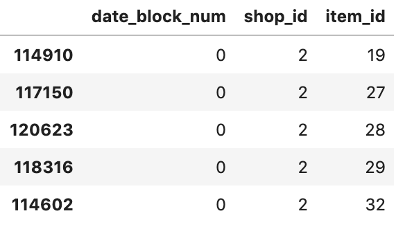
(월, 상점, 상품) 단위의 데이터프레임을 짰으니, 이제 이 단위로 월 세일즈량을 추가해줍시다.
극단 값에 robust 하게 하기 위해, 0~20 으로 범위를 맞춰주고,
결측치는 일단 0으로 채워줍니다.
ts = time.time()
group = train.groupby(['date_block_num','shop_id','item_id']).agg({'item_cnt_day': ['sum']})
group.columns = ['item_cnt_month']
group.reset_index(inplace=True)

matrix = pd.merge(matrix, group, on=cols, how='left')
matrix['item_cnt_month'] = (matrix['item_cnt_month']
                                .fillna(0)
                                .clip(0,20) # NB clip target here
                                .astype(np.float16))
time.time() - ts
matrix.head()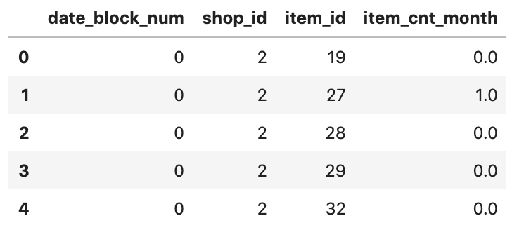
Test set
Test 데이터셋도, Train 데이터셋과 같은 꼴로 만들어주겠습니다.
test['date_block_num'] = 34
test['date_block_num'] = test['date_block_num'].astype(np.int8)
test['shop_id'] = test['shop_id'].astype(np.int8)
test['item_id'] = test['item_id'].astype(np.int16)
test.head()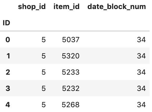
그리고 Test 데이터셋도 matrix 에 합쳐줍니다.
이로써, matrix 는 Train 과 Test 데이터셋을 모두 합친 데이터프레임이 됩니다.
앞으로 우리가 Feature 생성을 할 데이터프레임이기도 합니다.
ts = time.time()
matrix = pd.concat([matrix, test], ignore_index=True, sort=False, keys=cols)
matrix.fillna(0, inplace=True) # 34 month
time.time() - ts
matrix.head()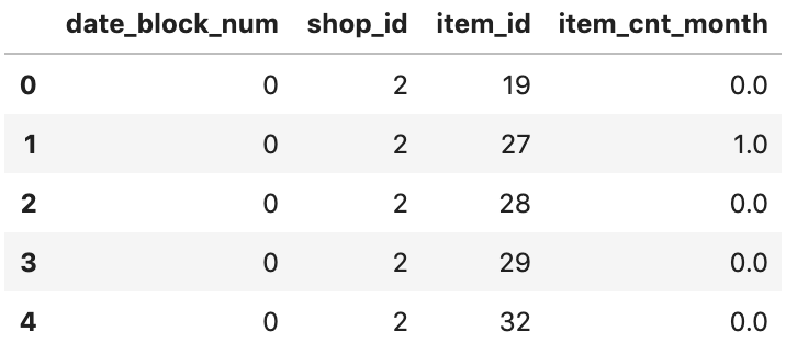
matrix.tail()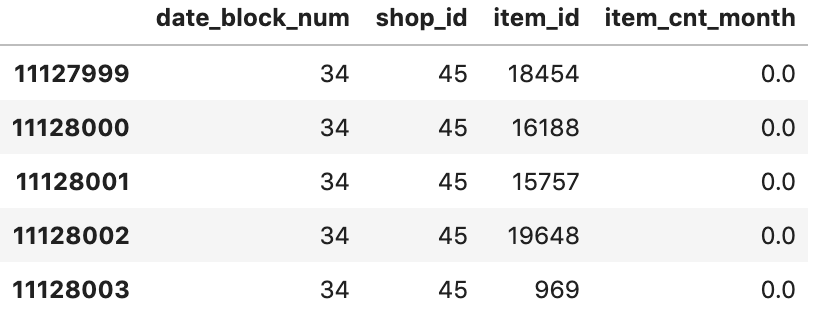
Shops/Items/Cats features
이제 본격적으로 Feature 들을 만들어보겠습니다.
제일 먼저, 이전에 만들었던 Feature 들,
즉, city_code, item_category_id, type_code, subtype_code 를 matrix의 feature 로 넣어줍니다.
ts = time.time()
matrix = pd.merge(matrix, shops, on=['shop_id'], how='left')
matrix = pd.merge(matrix, items, on=['item_id'], how='left')
matrix = pd.merge(matrix, cats, on=['item_category_id'], how='left')
matrix['city_code'] = matrix['city_code'].astype(np.int8)
matrix['item_category_id'] = matrix['item_category_id'].astype(np.int8)
matrix['type_code'] = matrix['type_code'].astype(np.int8)
matrix['subtype_code'] = matrix['subtype_code'].astype(np.int8)
time.time() - ts
matrix.head()
Traget lags
우리가 최종적으로 예측하려고하는 값은 '34번 째 달의 (월, 상점, 상품) 의 세일즈량' 임을 다시 상기해보겠습니다.
우리는 이 값을 이전 달들의 데이터를 가지고 예측해야 합니다.
따라서, 현재 해당 달의 이전 달들의 여러 값을(Lag) 을 현재 달의 Feature 로 둘 필요가 있습니다.
예를 들어, 34번째 달의 세일즈량 예측에 33번째 달과 32번째 달의 세일즈량을 Feature 로 둘 수 있습니다.
이런 방식으로 Feature 를 생성해보겠습니다.
def lag_feature(df, lags, col):
    """
    이전 달의 feature 들을, 현재 월의 feature 로 둡니다.
    이 떄, 이전 달들의 정보는 lags 에,
    사용할 feature 들은 col 에 담겨져 있습니다.
    """
    tmp = df[['date_block_num','shop_id','item_id',col]]
    for i in lags:
        shifted = tmp.copy()
        shifted.columns = ['date_block_num','shop_id','item_id', col+'_lag_'+str(i)]
        shifted['date_block_num'] += i
        df = pd.merge(df, shifted, on=['date_block_num','shop_id','item_id'], how='left')
    return df
ts = time.time()
# 1,2,3,6,12 달 전의 item_cnt_month 값을, 현재 해당 월의 feature 로 둡니다.
matrix = lag_feature(matrix, [1,2,3,6,12], 'item_cnt_month')
time.time() - tsmatrix.head()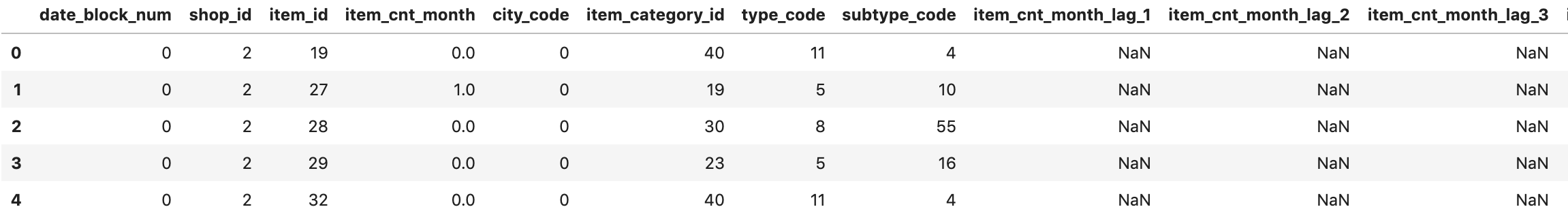
Mean encoded features
위와 같은 방식으로 여러 feature 값들을 생성합니다.
# 해당 월에, 일반적으로 상품들이 팔린 평균 개수 (즉, 월 단위로 같음.) 과 레그.
ts = time.time()
group = matrix.groupby(['date_block_num']).agg({'item_cnt_month': ['mean']})
group.columns = [ 'date_avg_item_cnt' ]
group.reset_index(inplace=True)

matrix = pd.merge(matrix, group, on=['date_block_num'], how='left')
matrix['date_avg_item_cnt'] = matrix['date_avg_item_cnt'].astype(np.float16)
matrix = lag_feature(matrix, [1], 'date_avg_item_cnt')
matrix.drop(['date_avg_item_cnt'], axis=1, inplace=True)
time.time() - ts
# 해당 월에, 각각의 상품 단위로, 팔린 상품 갯수의 평균 (즉, (월, 상품) 단위) 와 레그.
ts = time.time()
group = matrix.groupby(['date_block_num', 'item_id']).agg({'item_cnt_month': ['mean']})
group.columns = [ 'date_item_avg_item_cnt' ]
group.reset_index(inplace=True)
matrix = pd.merge(matrix, group, on=['date_block_num','item_id'], how='left')
matrix['date_item_avg_item_cnt'] = matrix['date_item_avg_item_cnt'].astype(np.float16)
matrix = lag_feature(matrix, [1,2,3,6,12], 'date_item_avg_item_cnt')
matrix.drop(['date_item_avg_item_cnt'], axis=1, inplace=True)
time.time() - ts# 해당 월에, 각각의 상점 단위로, 팔린 상품 갯수의 평균과 레그. (월, 상점) 단위
ts = time.time()
group = matrix.groupby(['date_block_num', 'shop_id']).agg({'item_cnt_month': ['mean']})
group.columns = [ 'date_shop_avg_item_cnt' ]
group.reset_index(inplace=True)
matrix = pd.merge(matrix, group, on=['date_block_num','shop_id'], how='left')
matrix['date_shop_avg_item_cnt'] = matrix['date_shop_avg_item_cnt'].astype(np.float16)
matrix = lag_feature(matrix, [1,2,3,6,12], 'date_shop_avg_item_cnt')
matrix.drop(['date_shop_avg_item_cnt'], axis=1, inplace=True)
time.time() - ts# 해당 월에, 각각의 아이템 카테고리 단위로, 팔린 상품 갯수의 평균과 레그. (월, 아이템 카테고리) 단위
ts = time.time()
group = matrix.groupby(['date_block_num', 'item_category_id']).agg({'item_cnt_month': ['mean']})
group.columns = [ 'date_cat_avg_item_cnt' ]
group.reset_index(inplace=True)
matrix = pd.merge(matrix, group, on=['date_block_num','item_category_id'], how='left')
matrix['date_cat_avg_item_cnt'] = matrix['date_cat_avg_item_cnt'].astype(np.float16)
matrix = lag_feature(matrix, [1], 'date_cat_avg_item_cnt')
matrix.drop(['date_cat_avg_item_cnt'], axis=1, inplace=True)
time.time() - ts# 해당 월에, 각각의 상점에서, 아이템 카테고리 단위로, 팔린 상품 갯수의 평균과 레그. (월, 상점, 아이템 카테고리) 단위
ts = time.time()
group = matrix.groupby(['date_block_num', 'shop_id', 'item_category_id']).agg({'item_cnt_month': ['mean']})
group.columns = ['date_shop_cat_avg_item_cnt']
group.reset_index(inplace=True)
matrix = pd.merge(matrix, group, on=['date_block_num', 'shop_id', 'item_category_id'], how='left')
matrix['date_shop_cat_avg_item_cnt'] = matrix['date_shop_cat_avg_item_cnt'].astype(np.float16)
matrix = lag_feature(matrix, [1], 'date_shop_cat_avg_item_cnt')
matrix.drop(['date_shop_cat_avg_item_cnt'], axis=1, inplace=True)
time.time() - ts# 해당 월에, 각각의 아이템 타입1 단위로, 팔린 상품 갯수의 평균과 레그. (월, 상점, 타입1) 단위
ts = time.time()
group = matrix.groupby(['date_block_num', 'shop_id', 'type_code']).agg({'item_cnt_month': ['mean']})
group.columns = ['date_shop_type_avg_item_cnt']
group.reset_index(inplace=True)
matrix = pd.merge(matrix, group, on=['date_block_num', 'shop_id', 'type_code'], how='left')
matrix['date_shop_type_avg_item_cnt'] = matrix['date_shop_type_avg_item_cnt'].astype(np.float16)
matrix = lag_feature(matrix, [1], 'date_shop_type_avg_item_cnt')
matrix.drop(['date_shop_type_avg_item_cnt'], axis=1, inplace=True)
time.time() - ts# 해당 월에, 각각의 아이템 타입2 단위로, 팔린 상품 갯수의 평균과 레그. (월, 상점, 타입2) 단위
ts = time.time()
group = matrix.groupby(['date_block_num', 'shop_id', 'subtype_code']).agg({'item_cnt_month': ['mean']})
group.columns = ['date_shop_subtype_avg_item_cnt']
group.reset_index(inplace=True)
matrix = pd.merge(matrix, group, on=['date_block_num', 'shop_id', 'subtype_code'], how='left')
matrix['date_shop_subtype_avg_item_cnt'] = matrix['date_shop_subtype_avg_item_cnt'].astype(np.float16)
matrix = lag_feature(matrix, [1], 'date_shop_subtype_avg_item_cnt')
matrix.drop(['date_shop_subtype_avg_item_cnt'], axis=1, inplace=True)
time.time() - ts# 해당 월에, 도시 단위로 팔린 상품 갯수의 평균과 레그 (월, 도시) 단위
ts = time.time()
group = matrix.groupby(['date_block_num', 'city_code']).agg({'item_cnt_month': ['mean']})
group.columns = [ 'date_city_avg_item_cnt' ]
group.reset_index(inplace=True)
matrix = pd.merge(matrix, group, on=['date_block_num', 'city_code'], how='left')
matrix['date_city_avg_item_cnt'] = matrix['date_city_avg_item_cnt'].astype(np.float16)
matrix = lag_feature(matrix, [1], 'date_city_avg_item_cnt')
matrix.drop(['date_city_avg_item_cnt'], axis=1, inplace=True)
time.time() - ts# 해당 월에, 각각 아이템, 도시 단위로, 팔린 상품 갯수의 평균과 레그. (월, 아이템, 도시) 단위
ts = time.time()
group = matrix.groupby(['date_block_num', 'item_id', 'city_code']).agg({'item_cnt_month': ['mean']})
group.columns = [ 'date_item_city_avg_item_cnt' ]
group.reset_index(inplace=True)
matrix = pd.merge(matrix, group, on=['date_block_num', 'item_id', 'city_code'], how='left')
matrix['date_item_city_avg_item_cnt'] = matrix['date_item_city_avg_item_cnt'].astype(np.float16)
matrix = lag_feature(matrix, [1], 'date_item_city_avg_item_cnt')
matrix.drop(['date_item_city_avg_item_cnt'], axis=1, inplace=True)
time.time() - ts# 해당 월에, 각각의 아이템 타입1 단위로, 팔린 상품 갯수의 평균과 레그. (월, 타입1) 단위
ts = time.time()
group = matrix.groupby(['date_block_num', 'type_code']).agg({'item_cnt_month': ['mean']})
group.columns = [ 'date_type_avg_item_cnt' ]
group.reset_index(inplace=True)
matrix = pd.merge(matrix, group, on=['date_block_num', 'type_code'], how='left')
matrix['date_type_avg_item_cnt'] = matrix['date_type_avg_item_cnt'].astype(np.float16)
matrix = lag_feature(matrix, [1], 'date_type_avg_item_cnt')
matrix.drop(['date_type_avg_item_cnt'], axis=1, inplace=True)
time.time() - ts# 해당 월에, 각각의 아이템 타입2 단위로, 팔린 상품 갯수의 평균과 레그. (월, 타입2) 단위
ts = time.time()
group = matrix.groupby(['date_block_num', 'subtype_code']).agg({'item_cnt_month': ['mean']})
group.columns = [ 'date_subtype_avg_item_cnt' ]
group.reset_index(inplace=True)
matrix = pd.merge(matrix, group, on=['date_block_num', 'subtype_code'], how='left')
matrix['date_subtype_avg_item_cnt'] = matrix['date_subtype_avg_item_cnt'].astype(np.float16)
matrix = lag_feature(matrix, [1], 'date_subtype_avg_item_cnt')
matrix.drop(['date_subtype_avg_item_cnt'], axis=1, inplace=True)
time.time() - tsfeature를 선정한 기준은, 주로 직관에 의존했거나 혹은 실험적으로 중요했던 feature 들을 골라 만들었습니다.
물론 이러한 feature 선정과 생성까지 단번에 되는 것은 아닙니다.
여러번의 실험과 시행착오 끝에 얻어진 코드라고 보시면 되겠습니다.
Trend features
이번엔 트랜드에 대한 Feature 를 만들어볼까 합니다.
여기서 트랜드란, 현재 달 기준, 지난 달의 특정 Feature 의 값이, 전체 평균보다 높은지 낮은지를 말합니다.
예를 들어, 지난 달의 특정 가게애서 어떤 상품의 가격이 전 기간동안의 가격 평균보다 높았다면, + 트랜드라고 말할 수 있습니다.
반대로 낮았다면, - 트랜드라고 말할 수 있습니다.
그런데 문제가 하나 있습니다.
만약 지난 달의 해당 상품의 매출이 없어서, Feature 값이 없는 경우(NaN)에는 어떻게 할까요?
이럴 경우, 2달 전의 Feature 값을 대신 사용합니다.
2달 전도 없는경우 3달 전, 또 없는 경우 4달전.. 이런 식으로 최대 6달 전까지 살펴보겠습니다.
먼저 상품 가격의 트랜드 Feature 를 만들어보겠습니다.
ts = time.time()

# 전 기간동안의 각각 상품의 평균 가격. (상품) 단위.
group = train.groupby(['item_id']).agg({'item_price': ['mean']})
group.columns = ['item_avg_item_price']
group.reset_index(inplace=True)

matrix = pd.merge(matrix, group, on=['item_id'], how='left')
matrix['item_avg_item_price'] = matrix['item_avg_item_price'].astype(np.float16)

# 월별 상품 평균 가격. (월, 상품) 단위.
group = train.groupby(['date_block_num','item_id']).agg({'item_price': ['mean']})
group.columns = ['date_item_avg_item_price']
group.reset_index(inplace=True)

matrix = pd.merge(matrix, group, on=['date_block_num','item_id'], how='left')
matrix['date_item_avg_item_price'] = matrix['date_item_avg_item_price'].astype(np.float16)

# 월별, 각 1~6개월 전의 평균 가격 (월, 상품) 단위.
lags = [1,2,3,4,5,6]
matrix = lag_feature(matrix, lags, 'date_item_avg_item_price')

# 월별, 각 1~6개월 전의 평균 가격과 전 기간 평균 가격과의 차이. (월, 상품) 단위.
# 전 구간 가격 평균하고 1~6달 가격을 비교함으로써, 지난 1~6달간의 가격 트랜드를 알 수 있음.
for i in lags:
    matrix['delta_price_lag_'+str(i)] = \
        (matrix['date_item_avg_item_price_lag_'+str(i)] - matrix['item_avg_item_price']) / matrix['item_avg_item_price']

# 현재 달 기준, 지난 1~6달 중, 최근의 트랜드를 찾음.
# 가장 최근 1달 전이 좋지만, 없을 경우 최대 6달 전까지 찾는 것.
def select_trend(row):
    for i in lags:
        if row['delta_price_lag_'+str(i)]:
            return row['delta_price_lag_'+str(i)]
    return 0

matrix['delta_price_lag'] = matrix.apply(select_trend, axis=1)
matrix['delta_price_lag'] = matrix['delta_price_lag'].astype(np.float16)
matrix['delta_price_lag'].fillna(0, inplace=True)

# feature drop 하기
# 가장 최근 price trend 를 찾았으니, 가격과 관련된 이전 lags 들은 필요 없음.
fetures_to_drop = ['item_avg_item_price', 'date_item_avg_item_price']
for i in lags:
    fetures_to_drop += ['date_item_avg_item_price_lag_'+str(i)]
    fetures_to_drop += ['delta_price_lag_'+str(i)]

matrix.drop(fetures_to_drop, axis=1, inplace=True)

time.time() - ts
이번엔, 해당 상점의 수입에 대한 트랜드를 Feature 로 만들겠습니다.
train['revenue'] = train['item_price'] * train['item_cnt_day']# 가격 트랜드와 동일하게, 총 수입 트랜드도 잡아봄.
# 가격 트랜드 방법과 똑같음.
ts = time.time()
# 월별 각각의 상점 총 매출. (월, 상점) 단위.
group = train.groupby(['date_block_num','shop_id']).agg({'revenue': ['sum']})
group.columns = ['date_shop_revenue']
group.reset_index(inplace=True)
matrix = pd.merge(matrix, group, on=['date_block_num','shop_id'], how='left')
matrix['date_shop_revenue'] = matrix['date_shop_revenue'].astype(np.float32)
# 전 기간동안, 각각의 상점 매출 평균. (상점) 단위.
group = group.groupby(['shop_id']).agg({'date_shop_revenue': ['mean']})
group.columns = ['shop_avg_revenue']
group.reset_index(inplace=True)
matrix = pd.merge(matrix, group, on=['shop_id'], how='left')
matrix['shop_avg_revenue'] = matrix['shop_avg_revenue'].astype(np.float32)
# 각각 상점의 월평균 매출 - 전기간 평균매출 의 차이. (월, 상점) 단위.
matrix['delta_revenue'] = (matrix['date_shop_revenue'] - matrix['shop_avg_revenue']) / matrix['shop_avg_revenue']
matrix['delta_revenue'] = matrix['delta_revenue'].astype(np.float16)
# 가장 최근 한 달전의 총 매출만 사용.
matrix = lag_feature(matrix, [1], 'delta_revenue')
# 최근 총매출 트랜드를 얻었으니, 필요없는 Feature들 다시 삭제.
matrix.drop(['date_shop_revenue','shop_avg_revenue','delta_revenue'], axis=1, inplace=True)
time.time() - tsSpecial features
지금까지 한 것 이외에, 별도의 Feature 들을 추가해보겠습니다.
다음의 Feature 들을 추가합니다.
- 월, 일
- (상점, 상품) 단위로, 해당 월 기준, 몇 달전에 마지막으로 팔렸는지.
- (상품) 단위로, 해당 월 기준, 몇 달전에 마지막으로 팔렸는지
- (상점, 상품) 단위로, 최초 판매 이후 개월.
- (상품) 단위로, 최초 판매 이후 개월.
matrix['month'] = matrix['date_block_num'] % 12

days = pd.Series([31,28,31,30,31,30,31,31,30,31,30,31])
matrix['days'] = matrix['month'].map(days).astype(np.int8)
여기서, 위에 2,3 번 Feature 를 만들기 위해, 다음과 같은 방법을 사용합니다.
- {(shop_id, item_id) : date_block_num} 꼴 모양의 해시테이블(dictonary)을 만듭니다. (3의 경우, (item_id) : date_block_num)
- 데이터 처음부터 루프문을 돕니다.
- 루프문 내, 각 데이터의 {row.shop_id, row.item_id} 가 해시테이블에 존재하지않으면, row.date_block_num의 값을 가지는 (row.shop_id, row.item_id)를 해시테이블에 추가합니다.
- 만약 해시테이블에 존재하면, 해시테이블에 존재하는 값과 현재 데이터의 row.date_block_num의 차이를 계산하여 값으로 넣습니다.
ts = time.time()
cache = {}
matrix['item_shop_last_sale'] = -1
matrix['item_shop_last_sale'] = matrix['item_shop_last_sale'].astype(np.int8)

# (상점, 상품)단위로, 해당 상품이 해당 월 기준, 몇 달전에 마지막으로 팔렸는지, item_shop_last_sale 에 저장.
# 예를 들어 1달 전에 팔렸으면 1임.
for idx, row in matrix.iterrows():
    key = str(row.item_id)+' '+str(row.shop_id)
    if key not in cache:
        if row.item_cnt_month != 0:
            cache[key] = row.date_block_num
    else:
        last_date_block_num = cache[key]
        matrix.at[idx, 'item_shop_last_sale'] = row.date_block_num - last_date_block_num
        cache[key] = row.date_block_num
time.time() - ts
ts = time.time()
cache = {}
matrix['item_last_sale'] = -1
matrix['item_last_sale'] = matrix['item_last_sale'].astype(np.int8)
# (상품) 단위로, 해당 상품이 해당 월 기준, 몇 달전에 마지막으로 팔렸는지, item_last_sale 에 저장.
for idx, row in matrix.iterrows():
key = row.item_id
if key not in cache:
if row.item_cnt_month != 0:
cache[key] = row.date_block_num
else:
last_date_block_num = cache[key]
if row.date_block_num > last_date_block_num:
matrix.at[idx, 'item_last_sale'] = row.date_block_num - last_date_block_num
cache[key] = row.date_block_num
time.time() - ts4번, 5번은 다음과 같이 얻습니다.
ts = time.time()

matrix['item_shop_first_sale'] = matrix['date_block_num'] - matrix.groupby(['item_id','shop_id'])['date_block_num'].transform('min')
matrix['item_first_sale'] = matrix['date_block_num'] - matrix.groupby('item_id')['date_block_num'].transform('min')
time.time() - ts
Final preparations
지금까지 전처리한 matrix 를 최종적으로 모델에 넣기 전에, 마지막 준비를 해보겠습니다.
먼저, 우리가 만든 feature 중에는, 해당 월의 12개월 전 데이터를 포함하는 값들이 있습니다.
예를 들어, date_item_avg_item_cnt_lag_12 와 같은 feature 입니다.
따라서, 데이터 초반 기준, 12개월 이후의 데이터부터 사용해야, 온전한 데이터 feature 값을 얻을 수 있을 것입니다.
ts = time.time()
matrix = matrix[matrix.date_block_num > 11]
time.time() - ts
또한, lags 관련 features 에서, 비어있는 값들을 0으로 채워줍니다.
ts = time.time()
def fill_na(df):
    for col in df.columns:
        if ('_lag_' in col) & (df[col].isnull().any()):
            if ('item_cnt' in col):
                df[col].fillna(0, inplace=True)
    return df

matrix = fill_na(matrix)
time.time() - ts
최종적으로, 어떤 features 가 있는지 확인해보겠습니다.
matrix.columnsIndex(['date_block_num', 'shop_id', 'item_id', 'item_cnt_month', 'city_code',
'item_category_id', 'type_code', 'subtype_code', 'item_cnt_month_lag_1',
'item_cnt_month_lag_2', 'item_cnt_month_lag_3', 'item_cnt_month_lag_6',
'item_cnt_month_lag_12', 'date_avg_item_cnt_lag_1',
'date_item_avg_item_cnt_lag_1', 'date_item_avg_item_cnt_lag_2',
'date_item_avg_item_cnt_lag_3', 'date_item_avg_item_cnt_lag_6',
'date_item_avg_item_cnt_lag_12', 'date_shop_avg_item_cnt_lag_1',
'date_shop_avg_item_cnt_lag_2', 'date_shop_avg_item_cnt_lag_3',
'date_shop_avg_item_cnt_lag_6', 'date_shop_avg_item_cnt_lag_12',
'date_cat_avg_item_cnt_lag_1', 'date_shop_cat_avg_item_cnt_lag_1',
'date_shop_type_avg_item_cnt_lag_1',
'date_shop_subtype_avg_item_cnt_lag_1', 'date_city_avg_item_cnt_lag_1',
'date_item_city_avg_item_cnt_lag_1', 'date_type_avg_item_cnt_lag_1',
'date_subtype_avg_item_cnt_lag_1', 'delta_price_lag',
'delta_revenue_lag_1', 'month', 'days', 'item_shop_last_sale',
'item_last_sale', 'item_shop_first_sale', 'item_first_sale'],
dtype='object')matrix.info()<class 'pandas.core.frame.DataFrame'>
Int64Index: 6639294 entries, 4488710 to 11128003
Data columns (total 40 columns):
date_block_num int8
shop_id int8
item_id int16
item_cnt_month float16
city_code int8
item_category_id int8
type_code int8
subtype_code int8
item_cnt_month_lag_1 float16
item_cnt_month_lag_2 float16
item_cnt_month_lag_3 float16
item_cnt_month_lag_6 float16
item_cnt_month_lag_12 float16
date_avg_item_cnt_lag_1 float16
date_item_avg_item_cnt_lag_1 float16
date_item_avg_item_cnt_lag_2 float16
date_item_avg_item_cnt_lag_3 float16
date_item_avg_item_cnt_lag_6 float16
date_item_avg_item_cnt_lag_12 float16
date_shop_avg_item_cnt_lag_1 float16
date_shop_avg_item_cnt_lag_2 float16
date_shop_avg_item_cnt_lag_3 float16
date_shop_avg_item_cnt_lag_6 float16
date_shop_avg_item_cnt_lag_12 float16
date_cat_avg_item_cnt_lag_1 float16
date_shop_cat_avg_item_cnt_lag_1 float16
date_shop_type_avg_item_cnt_lag_1 float16
date_shop_subtype_avg_item_cnt_lag_1 float16
date_city_avg_item_cnt_lag_1 float16
date_item_city_avg_item_cnt_lag_1 float16
date_type_avg_item_cnt_lag_1 float16
date_subtype_avg_item_cnt_lag_1 float16
delta_price_lag float16
delta_revenue_lag_1 float16
month int8
days int8
item_shop_last_sale int8
item_last_sale int8
item_shop_first_sale int8
item_first_sale int8
dtypes: float16(27), int16(1), int8(12)
memory usage: 481.2 MB메모리 절약을 하기위해, matrix 를 picklized 하고,
지금까지 전처리하는데 사용한 메모리들을 모두 free 해줍니다.
matrix.to_pickle('data.pkl')
del matrix
del cache
del group
del items
del shops
del cats
del train
# leave test for submission
gc.collect();
Part 2, xgboost
이제 본격적으로, 모델에 넣어보도록 하겠습니다.
먼저, picklized 한 데이터를 불러옵니다.
data = pd.read_pickle('data.pkl')실제로 사용할 features 입니다.
모델 feature 를 빼고싶을 때, 아래와 같이 주석처리만 해주면 됩니다.
feature를 넣고 빼는 일은, 모델을 여러번 평가할 때 사용하게 됩니다.
data = data[[
    'date_block_num',
    'shop_id',
    'item_id',
    'item_cnt_month',
    'city_code',
    'item_category_id',
    'type_code',
    'subtype_code',
    'item_cnt_month_lag_1',
    'item_cnt_month_lag_2',
    'item_cnt_month_lag_3',
    'item_cnt_month_lag_6',
    'item_cnt_month_lag_12',
    'date_avg_item_cnt_lag_1',
    'date_item_avg_item_cnt_lag_1',
    'date_item_avg_item_cnt_lag_2',
    'date_item_avg_item_cnt_lag_3',
    'date_item_avg_item_cnt_lag_6',
    'date_item_avg_item_cnt_lag_12',
    'date_shop_avg_item_cnt_lag_1',
    'date_shop_avg_item_cnt_lag_2',
    'date_shop_avg_item_cnt_lag_3',
    'date_shop_avg_item_cnt_lag_6',
    'date_shop_avg_item_cnt_lag_12',
    'date_cat_avg_item_cnt_lag_1',
    'date_shop_cat_avg_item_cnt_lag_1',
    #'date_shop_type_avg_item_cnt_lag_1',
    #'date_shop_subtype_avg_item_cnt_lag_1',
    'date_city_avg_item_cnt_lag_1',
    'date_item_city_avg_item_cnt_lag_1',
    #'date_type_avg_item_cnt_lag_1',
    #'date_subtype_avg_item_cnt_lag_1',
    'delta_price_lag',
    'month',
    'days',
    'item_shop_last_sale',
    'item_last_sale',
    'item_shop_first_sale',
    'item_first_sale',
]]
Validation strategy is 34 month for the test set, 33 month for the validation set and 13-33 months for the train.
0~32개월까지는 train 데이터 셋으로,
33개월은 validation 데이터 셋으로,
34개월은 test 데이터 셋으로 사용하겠습니다.
우리가 최종적으로 예측하고 제출해야하는 개월은 34개월입니다.
X_train = data[data.date_block_num < 33].drop(['item_cnt_month'], axis=1)
Y_train = data[data.date_block_num < 33]['item_cnt_month']
X_valid = data[data.date_block_num == 33].drop(['item_cnt_month'], axis=1)
Y_valid = data[data.date_block_num == 33]['item_cnt_month']
X_test = data[data.date_block_num == 34].drop(['item_cnt_month'], axis=1)
del data
gc.collect();ts = time.time()
model = XGBRegressor(
max_depth=8,
n_estimators=1000,
min_child_weight=300,
colsample_bytree=0.8,
subsample=0.8,
eta=0.3,
seed=42)
model.fit(
X_train,
Y_train,
eval_metric="rmse",
eval_set=[(X_train, Y_train), (X_valid, Y_valid)],
verbose=True,
early_stopping_rounds = 10)
time.time() - ts[0] validation_0-rmse:1.12439 validation_1-rmse:1.11692
Multiple eval metrics have been passed: 'validation_1-rmse' will be used for early stopping.
Will train until validation_1-rmse hasn't improved in 10 rounds.
[1] validation_0-rmse:1.08311 validation_1-rmse:1.08008
[2] validation_0-rmse:1.05061 validation_1-rmse:1.04917
[3] validation_0-rmse:1.00879 validation_1-rmse:1.02391
[4] validation_0-rmse:0.980837 validation_1-rmse:1.00304
[5] validation_0-rmse:0.959025 validation_1-rmse:0.985387
[6] validation_0-rmse:0.93963 validation_1-rmse:0.971881
[7] validation_0-rmse:0.922127 validation_1-rmse:0.959833
[8] validation_0-rmse:0.908155 validation_1-rmse:0.950422
[9] validation_0-rmse:0.897723 validation_1-rmse:0.942468
[10] validation_0-rmse:0.888247 validation_1-rmse:0.93696
[11] validation_0-rmse:0.880224 validation_1-rmse:0.932316
[12] validation_0-rmse:0.873818 validation_1-rmse:0.927516
[13] validation_0-rmse:0.867282 validation_1-rmse:0.923283
[14] validation_0-rmse:0.861212 validation_1-rmse:0.919724
[15] validation_0-rmse:0.856908 validation_1-rmse:0.918038
[16] validation_0-rmse:0.852811 validation_1-rmse:0.915969
[17] validation_0-rmse:0.849736 validation_1-rmse:0.914286
[18] validation_0-rmse:0.8467 validation_1-rmse:0.913197
[19] validation_0-rmse:0.844056 validation_1-rmse:0.911767
[20] validation_0-rmse:0.841502 validation_1-rmse:0.911191
[21] validation_0-rmse:0.839348 validation_1-rmse:0.910339
[22] validation_0-rmse:0.837345 validation_1-rmse:0.909736
[23] validation_0-rmse:0.835395 validation_1-rmse:0.908974
[24] validation_0-rmse:0.833743 validation_1-rmse:0.908285
[25] validation_0-rmse:0.832032 validation_1-rmse:0.90783
[26] validation_0-rmse:0.83 validation_1-rmse:0.908222
[27] validation_0-rmse:0.828996 validation_1-rmse:0.907708
[28] validation_0-rmse:0.82804 validation_1-rmse:0.90779
[29] validation_0-rmse:0.826955 validation_1-rmse:0.907744
[30] validation_0-rmse:0.825802 validation_1-rmse:0.907522
[31] validation_0-rmse:0.824672 validation_1-rmse:0.907686
[32] validation_0-rmse:0.82391 validation_1-rmse:0.907653
[33] validation_0-rmse:0.822871 validation_1-rmse:0.908175
[34] validation_0-rmse:0.821799 validation_1-rmse:0.908647
[35] validation_0-rmse:0.820883 validation_1-rmse:0.908539
[36] validation_0-rmse:0.820147 validation_1-rmse:0.908075
[37] validation_0-rmse:0.819353 validation_1-rmse:0.908319
[38] validation_0-rmse:0.818662 validation_1-rmse:0.908072
[39] validation_0-rmse:0.817673 validation_1-rmse:0.908095
[40] validation_0-rmse:0.816911 validation_1-rmse:0.908398
Stopping. Best iteration:
[30] validation_0-rmse:0.825802 validation_1-rmse:0.907522validation score 가 0.9까지 떨어진게 보입니다.
성공적으로 모델을 만들었습니다.
이제, test 데이터셋으로 예측하고, 예측된 값을 submission 파일에 써줍니다.
Y_pred = model.predict(X_valid).clip(0, 20)
Y_test = model.predict(X_test).clip(0, 20)

submission = pd.DataFrame({
    "ID": test.index,
    "item_cnt_month": Y_test
})
submission.to_csv('xgb_submission.csv', index=False)

# save predictions for an ensemble
pickle.dump(Y_pred, open('xgb_train.pickle', 'wb'))
pickle.dump(Y_test, open('xgb_test.pickle', 'wb'))
만들어진 모델의 feature 의 중요도를 살펴보면 다음과 같습니다.
plot_features(model, (10,14))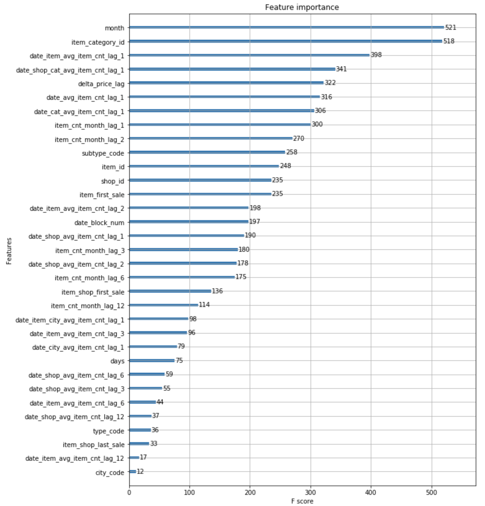
'데이터와 함께 탱고를 > 커널 공부하기' 카테고리의 다른 글
| [Predict Future Sales] playground 커널 리뷰 2 (0) | 2019.07.29 |
|---|---|
| [Predict Future Sales] playground 커널 리뷰 1 (2) | 2019.07.28 |
| [Predict Future Sales] playground 커널 리뷰 0 (0) | 2019.07.28 |
| [Predict Future Sales] 대회 및 데이터 소개 (1) | 2019.07.27 |
| 커널을 공부해본다. (0) | 2019.07.25 |


